Literature evaluate
Digital agriculture innovation administration
Digital agriculture includes the excellent digitization of agricultural worth chains, leveraging computational and communication applied sciences to equip farmers with enhanced data entry, progressive companies, and improved alternatives for boosting agricultural profitability and ecological sustainability9. First conceptualized in 1997, this paradigm represents technology-intensive farming methodologies augmented by geospatial techniques and superior data infrastructures10. This strategy integrates digital instruments and assets to optimize operational effectivity, improve financial viability for agricultural practitioners, and strengthen market competitiveness of farm merchandise by way of technological integration7. Academic consensus relating to digital agriculture’s conceptual boundaries stays elusive, and some scholarly consideration has expanded to embody digital infrastructure growth11, agricultural digitization processes12,13, and digital industrialization methods14. This rising tutorial engagement indicators digital transformation’s vital function in advancing agriculture towards high-quality financial growth.
The idea of AST innovation alliances lacks a universally accepted definition, with DAST innovation alliances representing an much more novel assemble. Functioning as a subset of commercial innovation alliances, these entities additionally embody strategic collaborative frameworks. The foundational notion of strategic alliances originated from Hopland (DEC Corporation’s former CEO) and administration scholar Nigel, who characterised them as collaborative entities fashioned by a number of enterprises sharing strategic aims and comparable operational capacities. Subsequent researchers refined this idea, describing strategic alliances as versatile cooperative preparations the place members leverage complementary strengths and risk-sharing mechanisms by way of contractual agreements to realize shared aims like market enlargement and useful resource optimization15. Contemporary analysis on AST innovation primarily examines 4 dimensions: innovation imperatives, methodological approaches, operational mechanisms, and strategic implementations. Pioneering work by researchers launched the induced technological innovation principle, positioning technological development because the central driver of agricultural progress16. Subsequent research have bolstered this attitude, with students emphasizing agricultural technological innovation’s vital function in sustaining trade growth and rural financial development17,18. Recent investigations highlighted collaborative partnerships between agricultural producers and Non-Governmental Organizations (NGOs) have been proven to boost specialised technology growth and knowledge-sharing networks amongst stakeholders19. Emerging analysis instructions embrace optimizing useful resource allocation methods for inexperienced agricultural innovation20 and analyzing diffusion mechanisms of agricultural technological developments by way of specialised innovation hubs like agricultural science parks21. These numerous scholarly efforts collectively contribute to our understanding of innovation dynamics in agricultural techniques, addressing each theoretical frameworks and sensible implementation challenges. We proposed articulate three particular dimensions that distinguish DAST alliances from standard strategic alliances, R&D consortia, and I-U-R collaborations: (a) Data-centric governance logic. Unlike conventional alliances the place useful resource complementarity includes bargaining over scarce belongings22, DAST alliances function on knowledge non-rivalry—agricultural knowledge may be concurrently utilized by a number of events with out depreciation, creating distinctive governance challenges round knowledge sovereignty, privateness, and worth attribution23. (b) Algorithmic co-production. While R&D consortia usually separate analysis and software phases, DAST alliances characteristic steady algorithmic iteration the place machine studying fashions are educated, validated, and refined by way of real-time agricultural knowledge streams, constituting a “living laboratory” innovation mode1. (c) Platform-based multilateralism. Traditional I-U-R collaborations are predominantly bilateral and project-bound. DAST alliances require multi-party knowledge interoperability throughout heterogeneous digital platforms (IoT gadgets, satellite tv for pc techniques, farm administration software program), necessitating novel requirements and API governance mechanisms.
Partner selection for innovation alliance
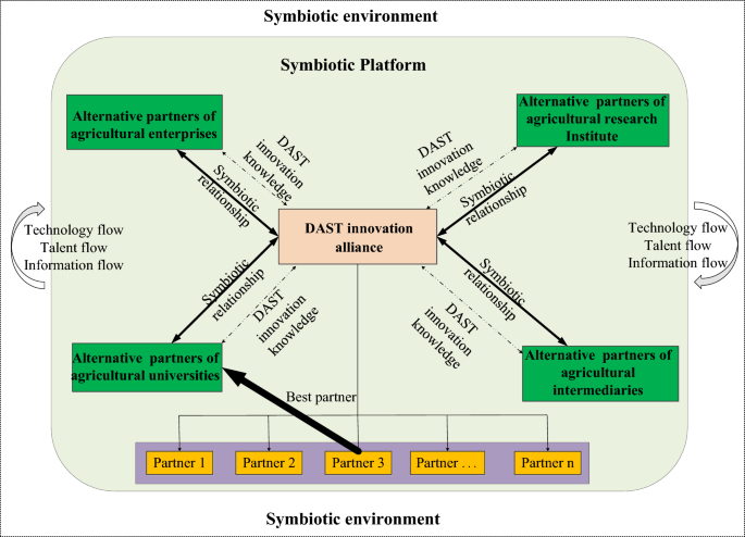
Drawing upon current analysis, this research posits that a DAST innovation alliance features as a collaborative entity the place dangers and rewards are collectively shared. Within such alliances, digital agriculture corporations, tutorial establishments, and analysis organizations collaborate on technological and product growth to entry mutually useful agricultural assets. The formation and longevity of such strategic innovation alliances essentially depend on enduring partnerships constructed on belief, with partner compatibility rising as a vital think about sustaining alliance stability24,25. Figure 1 illustrates the conceptual framework governing partner selection processes inside digital agricultural science and technology innovation alliances.

Theoretical mannequin of partner selection for DAST innovation alliance.
Within the digital agri-tech innovation consortium, agricultural enterprises, tutorial establishments, analysis organizations, and middleman businesses represent the core innovation actors. Collaborative interactions involving information switch, technological change, and data sharing between agricultural companies and tutorial establishments considerably improve the consortium’s progressive capability, as these partnerships facilitate the combination of numerous organizational competencies and specialised information techniques26,27. Through sustained collaboration in information dissemination, expertise cultivation, and technological development, innovation members regularly evolve into mutually useful relationships that allow complete sharing of complementary digital agricultural assets28,29. The institution of efficient symbiotic partnerships essentially is determined by members’ functionality to establish acceptable collaborators with aligned strategic aims30,31. While the consortium’s operational framework necessitates deciding on technical collaborators from a number of innovation entities, this partner selection course of includes intricate decision-making dynamics influenced by evolving technological necessities and market circumstances32,33.
MCDM issues and subject principle
Field principle constitutes a basic idea in physics, emphasizing the built-in and steady nature of spatial interactions that reveal imperceptible reciprocal relationships and dynamic influences34,35. This theoretical framework finds intensive functions throughout disciplines resembling chemistry, supplies science, biology, and medical analysis. Roe et al.36 systematically elaborated resolution subject principle whereas extending its implementation to numerous decision-making contexts. Song et al.37 innovatively built-in hesitation fuzzy units (HFS) with resolution subject principle (DFT) to ascertain a novel group resolution strategy termed hesitation fuzzy resolution subject principle (HFDFT) . Lee and Son38 subsequently merged the DFT paradigm with the DeGroot mannequin to create the superior DFT-L resolution structure. From the attitude of procedural resolution evaluation, Liu et al.39 formulated a multi-attribute group resolution methodology for dealing with incomplete linear ordered rating (ILOR) data based mostly on resolution subject ideas . The present research’s software of subject principle diverges from standard resolution subject approaches, providing vital insights into understanding useful resource complementarity, rational allocation, and compatibility optimization throughout partner selection processes.
Significant progress has been achieved in scholarly investigations relating to partner selection for industrial strategic alliances. These research have predominantly centered on two key dimensions: determinants affecting partnership decisions and methodological frameworks for analysis. Regarding influential elements, intensive analyses have examined dimensions resembling belief40, useful resource complementarity41, and collaborative compatibility42,43 in shaping alliance formation selections. Furthermore, tutorial explorations have built-in theoretical lenses together with information administration paradigms, synergy ideas, and sport principle fashions to not directly study partner selection dynamics by way of collaborative innovation motivations and incentive mechanisms. Notably, sure researchers have employed useful resource dependence principle to research how alliance partner selection and information acquisition methods influence innovation outcomes44, whereas others have developed selection frameworks emphasizing mission accountability and historic partnership efficiency45. In methodological developments, researchers have developed and refined numerous analytical frameworks, such because the DEMATEL-AEW-FVIOR hybrid strategy46, an built-in fuzzy MCDM framework combining LBWA (Level Based Weight Assessment) and Complex Proportional Assessment (COPRAS) technique47 and a hybrid Fuzzy Analytic Hierarchy Process—Combined Compromise Solution AHP-CoCoSo) mannequin48. In addition, researchers have launched novel decision-making frameworks. For occasion, Qiu et al.49 proposed two-stage mannequin employs the combination of Step-Wise Weight Assessment Ratio Analysis (SWARA) and Weighted Aggregated Sum Product Assessment (WASPAS) underneath spherical fuzzy (SF) circumstances to handle the strategic sequencing of sustainable insurance policies. Similarly, Chang et al.50 proposed a fuzzy delphi technique built-in with cluster evaluation. Golui et al.51 introduced a novel correlation coefficient for (FFSs), which includes the hesitancy operate into the calculation for the primary time. Bera et al.52 introduced a multi-criteria group decision-making (MCGDM) strategy by combining neutrosophic data with the Technique for Order of Preference by Similarity to Ideal Solution (TOPSIS) to resolve the MSME location selection difficulty. Current analysis limitations reveal that evaluations usually happen at remoted temporal factors by way of static analytical lenses, prioritizing optimum partner identification over alliance evolution. Notably, restricted consideration has been given to phased evaluations throughout a number of timeframes or dynamic partnership changes involving member transitions. Moreover, current scholarship insufficiently addresses the longitudinal nature of alliance partnerships and the cumulative results of iterative interactions between innovation networks and their constituent members.
Therefore, this analysis develops a dynamic partner selection framework for DAST innovation alliances by integrating dynamic intuitionistic fuzzy decision-making ideas with subject principle, emphasizing the evolving nature of collaborative innovation processes. The paper’s construction is organized into the next sections: part “Empirical research” formulates an alliance partner selection mechanism by way of subject principle functions, analyzing the logical consistency and sustainability when evaluating potential collaborators whereas establishing key withdrawal standards for current alliance members. Section “Discussion” demonstrates sensible implementation by way of China’s 5G Agricultural Digitalization Alliance case research, verifying the proposed methodology’s operational viability and sensible worth. The ultimate part (part “Conclusion“) synthesizes analysis findings, discusses theoretical contributions and managerial insights, and outlines potential instructions for future investigation.
Research framework
This a number of attribute decision-making (MADM) drawback includes two partner panels: various cooperation innovation companions and the companions in a longtime DAST innovation alliance. The set of the companions within the established DAST innovation alliance is denoted as (RT{textual content{ = { }}RT_{1} ,RT_{2} , cdots ,RT_{m} {textual content{} }}), and the set of the choice cooperation innovation companions is denoted as (S=left{ {S_{1} ,S_{2} ,…,S_{m} } proper}). The selection of companions for the DAST innovation alliance is a MADM drawback, and the factors set is represented as (G = left{ {G_{1} ,G_{2} ,…,G_{n} } proper}),(T = left{ {t_{1} ,t_{2} ,…,t_{okay} } proper}), which is a set of resolution levels composed of (okay) resolution durations. In totally different resolution durations (t_{okay}), the attribute worth of the (S_{i}) scheme underneath the attribute (G_{j}) is represented by an intuitionistic fuzzy quantity, denoted as (alpha_{ij}^{okay} = (mu_{ij}^{okay} ,upsilon_{ij}^{okay} )). Hence, the intuitionistic fuzzy resolution matrix of a resolution interval (t_{okay}) may be expressed as:
$$start{gathered} A(t_{okay} ) = (alpha_{ij}^{okay} )_{m occasions n} = (mu_{ij}^{okay} ,upsilon_{ij}^{okay} )_{m occasions n} = left[ {begin{array}{*{20}c} {(mu_{11}^{k} ,upsilon_{11}^{k} )} & {(mu_{12}^{k} ,upsilon_{12}^{k} )} & {…} & {(mu_{1n}^{k} ,upsilon_{1n}^{k} )} {(mu_{21}^{k} ,upsilon_{21}^{k} )} & {(mu_{22}^{k} ,upsilon_{22}^{k} )} & ldots & {(mu_{2n}^{k} ,upsilon_{2n}^{k} )} vdots & vdots & ddots & vdots {(mu_{m1}^{k} ,upsilon_{m1}^{k} )} & {(mu_{m2}^{k} ,upsilon_{m2}^{k} )} & ldots & {(mu_{mn}^{k} ,upsilon_{mn}^{k} )} end{array} } right] finish{gathered}$$
The weight of attributes in numerous time durations is totally different. The weight vector of attributes within the (okay) time interval is unknown, denoted as (omega^{okay} = (omega_{1}^{okay} ,omega_{2}^{okay} ,…,omega_{n}^{okay} )^{T}), the place (omega_{j}^{okay} in [0,1],sumlimits_{j = 1}^{n} {omega_{j}^{okay} } = 1). In this paper, the gray relational diploma technique and intuitionistic fuzzy entropy technique are mixed to resolve the attribute weight. The time weight vector can be unknown, denoted as (eta_{{t_{okay} }} = (eta (t_{1} ),eta (t_{2} ),…,eta (t_{p} ))^{T}), which displays the significance hooked up to totally different time durations within the decision-making course of, the place (eta (t_{okay} ) in [0,1])(,sumlimits_{okay = 1}^{p} {eta (t_{okay} )} = 1), (eta (t_{okay} )) is the load of the (okay)th time interval. In this paper, based mostly on the precept of most entropy, a nonlinear programming mannequin is established to resolve the temporal weight vector. Then the orthogonal projection technique is used to guage the alternate options comprehensively. In the precise DAST innovation, the complementary useful resource set between the members and various members of the innovation alliance is expressed as YR = (YR1 … YRl). Then, based mostly on the complementary useful resource a subject principle mannequin is built-in to pick out the DAST partner.
To set up the analysis framework for DAST alliance partner selection, the ideas of static attributes and dynamic competencies derived from subject principle are integrated to evaluate collaborative innovation potential. From the attitude of subject principle, potential alliance members exhibit twin dimensions: inherent qualities representing their steady traits, and developmental capabilities indicating their potential for integration into DAST innovation networks. The selection course of emphasizes three vital dimensions: useful resource synergy, collaborative information switch, and organizational alignment53. Through synthesis of current scholarship and evaluation of DAST alliance traits, the partner analysis system includes 5 core standards: useful resource complementary stage of a partner54,55, knowledge-sharing stage53,56, the cultural similarity of a partner57,58, and risk-sharing potential59, cooperation compatibility potential60. Figure 2 reveals the partner selection index framework of the DAST innovation alliance based mostly on the above theoretical framework.

The index framework of partner selection for DAST innovation alliance based mostly on the sector principle.
Preliminary
Intuitionistic fuzzy units (IFSs)
Definition 1
61Let a set (X = { x_{1} ,x_{2} , cdots x_{n} }) be a finite universe of discourse, then the set (A = { }) is an intuitionistic fuzzy set, the place, (u_{A} (x)) and (v_{A} (x)) are the membership diploma and non-membership diploma of the ingredient (x) in (X) belonging to (A), respectively: (mu_{A} (x):X to left[ {0,1} right]),(upsilon_{A} (x):X to left[ {0,1} right]), and (0 le mu_{A} (x) + upsilon_{A} (x) le 1,x in X).Besides, (pi_{A} = 1 – mu_{A} (x) – upsilon_{A} (x)) is the diploma of indeterminacy of (x) in (X) belonging to (A).
Definition 2
61Let (alpha_{1} = (mu_{{alpha_{1} }} ,nu_{{alpha_{1} }} )) and (alpha_{2} = (mu_{{alpha_{2} }} ,nu_{{alpha_{2} }} )) be two IFNs, (lambda) be a actual quantity, and (lambda > 0), then
-
1.
(alpha_{1} oplus alpha_{2} = (mu_{{alpha_{1} }} + mu_{{alpha_{2} }} – mu_{{alpha_{1} }} mu_{{alpha_{2} }} ,nu_{{alpha_{1} }} nu_{{alpha_{2} }} );)
-
2.
(alpha_{1} otimes alpha_{2} = (mu_{{alpha_{1} }} mu_{{alpha_{2} }} ,nu_{{alpha_{1} }} + nu_{{alpha_{2} }} – nu_{{alpha_{1} }} nu_{{alpha_{2} }} );)
-
3.
(lambda alpha_{1} = (1 – (1 – mu_{{alpha_{1} }} )^{lambda } ,nu_{{alpha_{1} }}^{lambda } );)
-
4.
(alpha_{{1}}^{lambda } = left( {mu_{{alpha_{{1}} }}^{lambda } ,1 – left( {1 – nu_{{alpha_{{1}} }}^{{}} } proper)^{lambda } } proper).)
Definition 3
62Let (alpha_{j} = (mu_{{A_{j} }} (x),nu_{{A_{j} }} (x)),j = 1,2,…,n,) be an IFN, then
$$IFWA_{omega } (alpha_{1} ,alpha_{2} ,…,alpha_{n} ) = sumlimits_{j = 1}^{n} {omega_{j} alpha_{j} = (1 – prodlimits_{j = 1}^{n} {left( {1 – mu_{{A_{j} }} (x)} proper)^{{omega_{j} }} } } ,prodlimits_{j = 1}^{n} {nu_{{A_{j} }} (x)^{{omega_{j} }} } )$$
is an intuitionistic fuzzy weighted averaging (IFWA) operator. Where, (IFWA:Q^{n} to Q),(omega { = }left( {omega_{1} omega_{2} …,omega_{n} } proper)^{T} ,omega_{j} ge 0),(j{ = }1,2,…,n),(sumnolimits_{j = 1}^{n} {omega_{j} } = 1.)
Definition 4
63Let (X = left{ {x_{1} ,x_{2} ,…,x_{n} } proper}) be a finite universe of discourse and (T = left{ {t_{1} ,t_{2} ,…,t_{p} } proper}) be a discrete time set. A dynamic intuitionistic fuzzy set (DIFS) (tilde{A}) in (X) is outlined as: (tilde{A} = left{ {leftlangle {x,u_{{tilde{A}}} (x,t),v_{{tilde{A}}} (x,t)} rightrangle left| {x in X,t in T} proper.} proper}). Where (u_{{tilde{A}}} (x,t):X occasions T to [0,1]) denotes the membership operate, (v_{{tilde{A}}} (x,t):X occasions T to [0,1]) denotes the non-membership operate, satisfying the situation:(0 le u_{{tilde{A}}} (x,t) + v_{{tilde{A}}} (x,t) le 1,forall x in X,t in T), the hesitation margin at time t is outlined as:(pi_{{tilde{A}}} (x,t) = {1 – }u_{{tilde{A}}} (x,t){ – }v_{{tilde{A}}} (x,t)), representing the diploma of uncertainty or indeterminacy evolving over time.
Definition 5
63Let t be a timing variable, then (alpha (t) = left( {mu_{alpha (t)} (x),nu_{alpha (t)} (x)} proper)) is an IFN, the place (mu_{alpha (t)} (x) in left[ {0,1} right],nu_{alpha (t)} (x) in left[ {0,1} right]),(mu_{alpha (t)} (x){ + }nu_{alpha (t)} (x) le 1), if (t{ = }t_{1} t_{2} …,t_{n}), and (alpha (t_{1} ),alpha (t_{2} ),…,alpha (t_{p} )) is outlined as p IFSs with totally different durations.
Definition 6
63Let (alpha_{{t_{okay} }} = (mu_{{t_{okay} }} ,nu_{{t_{okay} }} ))(left( {okay{ = }1,2,…,p} proper)) be an IFN at interval (t_{okay}), and (eta (t_{okay} ) = (eta (t_{1} )eta (t_{2} )…,eta (t_{p} ))^{T}) be the load vector of the time interval (t_{okay}), then
$$DIFWG_{eta (t)} (alpha_{{t_{1} }} ,alpha_{{t_{2} }} ,…,alpha_{{t_{p} }} ) = prodlimits_{okay = 1}^{p} {alpha_{{t_{okay} }}^{{eta (t_{okay} )}} } = (prodlimits_{okay = 1}^{p} {mu_{{t_{okay} }}^{{eta (t_{okay} )}} } ,1 – prodlimits_{okay = 1}^{p} {(1 – nu_{{t_{okay} }} } )^{{eta (t_{okay} )}} )$$
is a dynamic intuitionistic fuzzy weighted (DIFWG) operator, the place, (eta (t_{okay} ) in left[ {0,1} right],sumnolimits_{okay = 1}^{p} {eta (t_{okay} )} = 1)(left( {okay{ = }12…,p} proper).)
Definition 7
63Let (alpha_{1} = (mu_{{alpha_{1} }} ,nu_{{alpha_{1} }} )) and (alpha_{2} = (mu_{{alpha_{2} }} ,nu_{{alpha_{2} }} )) be two IFSs, then the Euclidean distance of the 2 IFSs is:
$$d(alpha_{1} ,alpha_{2} ) = sqrt[{}]{{frac{1}{2}left[ {left( {mu_{{alpha_{1} }} – mu_{{alpha_{2} }} } right)^{2} + left( {nu_{{alpha_{1} }} – nu_{{alpha_{2} }} } right)^{2} + left( {pi_{{alpha_{1} }} – pi_{{alpha_{2} }} } right)^{2} } right]}}$$
the place (pi_{{alpha_{i} }} = 1 – mu_{{alpha_{i} }} – nu_{{alpha_{i} }} ,(i = 1,2).)
Determination of attribute weights
In the fuzzy multi-attribute decision-making framework, establishing cheap attribute weights performs a pivotal function in making certain resolution high quality. This research proposes an built-in weighting method that mixes grey correlation evaluation with the utmost deviation strategy to find out attribute significance. The hybrid methodology concurrently considers decision-makers’ experiential judgments and quantitative knowledge traits, successfully mitigating potential biases from subjective assumptions whereas stopping over-reliance on data system outputs. This methodology balances decision-makers’ subjective preferences with the aims derived from decision-related knowledge, thereby enhancing the robustness of weight willpower by way of complementary analytical views.
Grey relational evaluation addresses decision-making challenges underneath circumstances of incomplete data and restricted knowledge factors. This methodology assesses interconnections amongst system variables whereas quantifying their mutual impacts. The method’s basis, as outlined by Wei64, examines geometric similarities in knowledge sequence curves from experimental samples to find out relational proximity.
The constructive and adverse excellent options for every attribute at time interval (okay) may be expressed as (A_{j}^{ + okay} = (alpha_{1}^{ + okay} ,alpha_{2}^{ + okay} ,…,alpha_{n}^{ + okay} )) and (A_{j}^{ – okay} = (alpha_{1}^{ – okay} ,alpha_{2}^{ – okay} ,…,alpha_{n}^{ – okay} )), respectively, the place
$$alpha_{j}^{ + okay} = (mu_{j}^{ + okay} ,upsilon_{j}^{ + okay} ) = (mathop {max}limits_{1 le i le m} mu_{ij}^{okay} ,mathop {min}limits_{1 le i le m} upsilon_{ij}^{okay} ),(j = 1,2,…,n)$$
(1)
$$alpha_{j}^{ – okay} = (mu_{j}^{ – okay} ,upsilon_{j}^{ – okay} ) = (mathop {min}limits_{1 le i le m} mu_{ij}^{okay} ,mathop {max}limits_{1 le i le m} upsilon_{ij}^{okay} ),(j = 1,2,…,n)$$
(2)
According to Definition 6, in time interval (okay), the space between a resolution and its correlated constructive excellent resolution is (d_{ij}^{ + } (A_{ij}^{okay} ,A_{j}^{ + okay} )), and the space between a resolution and its correlated adverse excellent resolution is (d_{ij}^{ – } (A_{ij}^{okay} ,A_{j}^{ – okay} )). Then, the correlation coefficients of the (i) th resolution with the constructive and adverse excellent options underneath attribute (j) in time interval (okay) may be calculated as follows:
$$varepsilon_{ij}^{ + okay} = frac{{mathop {min}limits_{i} mathop {min}limits_{j} d_{ij}^{ + } (A_{ij}^{okay} ,A_{j}^{ + okay} ) + rho mathop {max}limits_{i} mathop {max}limits_{j} d_{ij}^{ + } (A_{ij}^{okay} ,A_{j}^{ + okay} )}}{{d_{ij}^{ + } (A_{ij}^{okay} ,A_{j}^{ + okay} ) + rho mathop {max}limits_{i} mathop {max}limits_{j} d_{ij}^{ + } (A_{ij}^{okay} ,A_{j}^{ + okay} )}}$$
(3)
$$varepsilon_{ij}^{ – okay} = frac{{mathop {min}limits_{i} mathop {min}limits_{j} d_{ij}^{ – } (A_{ij}^{okay} ,A_{j}^{ – okay} ) + rho mathop {max}limits_{i} mathop {max}limits_{j} d_{ij}^{ – } (A_{ij}^{okay} ,A_{j}^{ – okay} )}}{{d_{ij}^{ – } (A_{ij}^{okay} ,A_{j}^{ – okay} ) + rho mathop {max}limits_{i} mathop {max}limits_{j} d_{ij}^{ – } (A_{ij}^{okay} ,A_{j}^{ – okay} )}}$$
(4)
the place (rho) is the distinguishing coefficient and (rho in [0,1]), and typically, (rho) is about to 0.5.
(chi^{okay} = (chi_{1}^{okay} ,chi_{2}^{okay} ,…,chi_{m}^{okay} )) is outlined because the attribute weight vector in time interval (okay), and (chi_{j}^{okay} in [0,1],sumlimits_{j = 1}^{m} {chi_{j}^{okay} } = 1(okay = 1,2,…,p)). As the correlation coefficient vector of a resolution and its constructive excellent resolution at time interval (okay) is ((1,1,…,1)), the sum of composite deviations of the correlation diploma between the (i) th resolution and its constructive excellent resolution in time interval (okay) is
$$gamma_{i}^{okay} (chi^{okay} ) = sumlimits_{j = 1}^{m} {[(1 – varepsilon_{ij}^{ + k} )} chi_{j}^{k} ]^{2}$$
(5)
Hence, a nonlinear programming mannequin, (M–1), may be constructed to reduce the sum of composite deviations of the correlation diploma between all options and their correlated constructive excellent options:
$$(M – 1)left{ {start{array}{*{20}c} {mingamma^{okay} (chi^{okay} ) = sumlimits_{i = 1}^{n} {sumlimits_{j = 1}^{m} {[(1 – varepsilon_{ij}^{ + k} )} chi_{j}^{k} ]^{2} } } {s.t.sumlimits_{j = 1}^{m} {chi_{j}^{okay} } = 1(okay = 1,2,…,p)} finish{array} } proper.$$
The resolution of (M–1) is
$$left{ {start{array}{*{20}l} {start{array}{*{20}l} {lambda = – [sumlimits_{j = 1}^{m} {(sumlimits_{i = 1}^{n} {(1 – varepsilon_{ij}^{ + k} )^{2} )^{ – 1} ]^{ – 1} } } } hfill {chi_{j}^{okay} = [sumlimits_{j = 1}^{m} {(sumlimits_{i = 1}^{n} {(1 – varepsilon_{ij}^{ + k} )^{2} )^{ – 1} ]^{ – 1} } } occasions [sumlimits_{i = 1}^{n} {(1 – varepsilon_{ij}^{ + k} )^{2} ]^{ – 1} } } hfill finish{array} } hfill finish{array} } proper.$$
(6)
On the opposite hand, taking the distinction of decision-making data underneath time collection traits and the desire of decision-makers towards every attribute in numerous durations under consideration, the intuitionistic fuzzy entropy technique is used to find out the load of every attribute underneath time collection63.
In time interval (t_{okay}), the intuitionistic fuzzy entropy of the attribute is
$$E_{j}^{okay} = frac{1}{m}sumlimits_{i = 1}^{m} {left{ {1 – sqrt {left( {1 – pi_{ij}^{okay} } proper)^{2} – mu_{ij}^{okay} nu_{ij}^{okay} } } proper}}$$
(7)
Set (phi_{j}^{okay}) because the attribute weight of the time interval (t_{okay}), an optimization mannequin of attribute weight within the time interval (t_{okay}), (M–2), is established as follows:
$$(M – 2)left{ {start{array}{*{20}c} {min sumlimits_{j = 1}^{n} {left( {phi_{j}^{okay} } proper)^{2} } E_{j}^{okay} } {s.tsumlimits_{j = 1}^{n} {phi_{j}^{okay} = 1} } finish{array} } proper.$$
After fixing mannequin (M–2), the load of the attribute may be obtained:
$$phi_{j}^{okay} = frac{{left( {E_{j}^{okay} } proper)^{ – 1} }}{{sumlimits_{j = 1}^{n} {left( {E_{j}^{okay} } proper)^{ – 1} } }}$$
(8)
Therefore, by combining the gray correlation evaluation technique and the intuitionistic fuzzy entropy technique, the load vector of complete attributes may be expressed as Eq. (9).
$$omega_{j} (t_{okay} ) = eta chi_{j}^{okay} { + }(1 – eta )phi_{j}^{okay} (okay = 1,2,…,p)$$
(9)
the place (omega_{j} (t_{okay} )) is the load vector of complete attributes within the time interval of (okay), and (omega_{j} (t_{okay} )) captures the aggressive precedence of analysis dimension j within the alliance’s present lifecycle stage. Usually, weight distribution patterns diagnose alliance strategic orientation and decision-makers establish useful resource allocation misalignment.(eta (0 le eta le 1)) is the expertise issue. Generally, (eta { = }0.5).
Determination of time weights
Definition 8
65Let (theta = sumlimits_{okay = 1}^{p} {frac{p – okay}{{p – 1}}eta (t_{okay} )}), and (theta in [0,1]), then (theta) is the time diploma of time sequence weight vector: (eta_{{t_{okay} }} = (eta (t_{1} ),eta (t_{2} ),…,eta (t_{p} ))^{T}). (eta (t_{okay} )) represents the strategic relevance depth of historic data for present decision-making. A better (eta (t_{okay} )) signifies that interval t’s alliance efficiency carries higher studying worth for predicting future trajectories.
Time diploma displays a decision-maker’s desire diploma in the direction of time collection, and the decision-makers typically give (theta) worth based mostly on expertise and desire. When (theta) developments to 0, it signifies that the decision-maker prefers latest data; when θ tends to 1, it implies that the decision-maker prefers previous data.
Information entropy quantifies the temporal weight vector’s capability to assimilate data quantity. Higher entropy values correspond to diminished data content material, with this relationship being mathematically represented by way of Eq. (10).
$$f(eta (t_{okay} )) = – sumlimits_{okay = 1}^{p} {eta (t_{okay} )ln eta (t_{okay} ),okay = 1} ,2,…,p$$
(10)
According to Definition 8, (eta_{{t_{okay} }} = (0,0,…,1)^{T}), (theta = 0) signifies a decision-maker fully prefers latest data, and the constructive excellent time weight vector is denoted as (eta_{{t_{okay} }}^{ + } = (0,0,…,1)^{T});(eta_{{t_{okay} }} = (1,0,…,0)^{T}),(theta = 1) signifies a decision-maker fully prefers previous data, and the adverse excellent time weight vector is denoted as (eta_{{t_{okay} }}^{ – } = (1,0,…,0)^{T}).
The distance between the 2 time weight vectors, (underline{eta }_{{t_{okay} }} = (underline{eta } (t_{1} ),underline{eta } (t_{2} ),…,underline{eta } (t_{p} ))^{T}) and (overline{eta }_{{t_{okay} }} = (overline{eta }(t_{1} ),overline{eta }(t_{2} ),…,overline{eta }(t_{p} ))^{T}), is about to be
$$d(underline{eta }_{{t_{okay} }} ,overline{eta }_{{t_{okay} }} ) = sqrt {sumlimits_{okay = 1}^{p} {(underline{eta } (t_{okay} ) – overline{eta }(t_{okay} ))^{2} } }$$
(11)
The separation between a temporal weight vector (eta_{{t_{okay} }} = (eta (t_{1} ),eta (t_{2} ),…,eta (t_{p} ))^{T}) and its related constructive excellent temporal weight vectors, together with the interval between the load vector and the associated adverse excellent temporal weight vectors, may be decided as follows:
$$d(eta_{{t_{okay} }} ,eta_{{t_{okay} }}^{ + } ) = sqrt {sumlimits_{okay = 1}^{p – 1} {eta (t_{okay} )^{2} + (1 – eta (t_{p} ))^{2} } }$$
(12)
$$d(eta_{{t_{okay} }} ,eta_{{t_{okay} }}^{ – } ) = sqrt {(1 – eta (t_{1} ))^{2} + sumlimits_{okay = 2}^{p} {eta (t_{okay} )^{2} } }$$
(13)
Hence, a nonlinear multi-objective programming mannequin, (M-3), is constructed by maximizing the flexibility of knowledge uptake, maximizing the closeness diploma to constructive excellent time weight vector, and minimizing the closeness diploma to the adverse excellent time weight vector:
$$(M – 3)left{ {start{array}{*{20}l} {maxbegin{array}{*{20}c} {} finish{array} f(eta (t_{okay} )) = – sumlimits_{okay = 1}^{p} {eta (t_{okay} )ln eta (t_{okay} )} } hfill start{gathered} maxbegin{array}{*{20}c} {} finish{array} d(eta_{{t_{okay} }} ,eta_{{t_{okay} }}^{ – } ) = sqrt {(1 – eta (t_{1} ))^{2} + sumlimits_{okay = 2}^{p} {eta (t_{okay} )^{2} } } hfill minbegin{array}{*{20}c} {} finish{array} d(eta_{{t_{okay} }} ,eta_{{t_{okay} }}^{ + } ) = sqrt {sumlimits_{okay = 1}^{p – 1} {eta (t_{okay} )^{2} + (1 – eta (t_{p} ))^{2} } } hfill finish{gathered} hfill {s.t.{kern 1pt} {kern 1pt} {kern 1pt} {kern 1pt} theta = sumlimits_{okay = 1}^{p} {frac{p – okay}{{p – 1}}eta (t_{okay} ),{kern 1pt} {kern 1pt} sumlimits_{okay = 1}^{p} {eta (t_{okay} ) = 1,eta (t_{okay} ) in left[ {0,1} right],okay = 1,2,..,p} } } hfill finish{array} } proper.$$
To simplify the calculation, this multi-objective optimization mannequin is remodeled into a single-objective optimization mannequin, (M-4):
$$(M – 4)left{ {start{array}{*{20}l} {minbegin{array}{*{20}c} {} finish{array} g = csqrt {sumlimits_{okay = 1}^{p – 1} {eta (t_{okay} )^{2} + (1 – eta (t_{p} ))^{2} } } – csqrt {(1 – eta (t_{1} ))^{2} + sumlimits_{okay = 2}^{p} {eta (t_{okay} )^{2} } } + (1 – 2c)(sumlimits_{okay = 1}^{p} {eta (t_{okay} )ln eta (t_{okay} )} )} hfill {s.t.{kern 1pt} {kern 1pt} {kern 1pt} {kern 1pt} theta = sumlimits_{okay = 1}^{p} {frac{p – okay}{{p – 1}}eta (t_{okay} ),{kern 1pt} {kern 1pt} sumlimits_{okay = 1}^{p} {eta (t_{okay} ) = 1,eta (t_{okay} ) in left[ {0,1} right],okay = 1,2,..,p} } } hfill finish{array} } proper.$$
the place (c) is the equilibrium coefficient, (c in [0,0.5]). Model (M-4) is solved utilizing Lingo 11.0 software program, and a time collection weight vector, (eta_{{t_{okay} }} = (eta (t_{1} ),eta (t_{2} ),…,eta (t_{p} ))^{T}), is obtained.
Orthogonal projection technique
The orthogonal projection technique was proposed by Hua et al.66 in 2004. In this technique, a vertical distance is outlined as the space between planes whose regular vectors are the traces connecting the constructive and adverse excellent options, respectively, between the constructive and adverse excellent options66. This primary content material is to beat the constraints of the Euclidean distance within the TOPSIS technique, serving as a substitute for the Euclidean distance to find out the closeness of alternate options.
To set up a vivid description of the vertical distance, the three-dimensional house is taken for example (see Fig. 3). P and (textual content{Q}) are the comparatively constructive and adverse excellent schemes amongst all alternate options. The distance between the airplane passes by way of the (textual content{X}) level with the straight line (textual content{PQ}) as the traditional vector and the airplane passes the (textual content{Y}) level with the straight line (textual content{PQ}) as the traditional vector, that’s, the space between the planes (textual content{L}) and (textual content{M}). This distance is the Euclidean distance between the orthogonal projection factors (textual content{O}) and (textual content{U}) on the road (textual content{PQ}) of factors (textual content{X}) and (textual content{Y}). Suppose the vectors similar to factors (textual content{P}), (textual content{Q}), (textual content{X}), (textual content{Y}) are (textual content{p}), (textual content{q}), (textual content{x}), (textual content{y}); then, the vertical distance between factors (textual content{X}) and (textual content{Y}) is
$$V = frac{{left| {(p – q) cdot (x – y)} proper|}}{{left| {p – q} proper|}}$$
(14)
In the components, (cdot) is the purpose multiplication of the vector; (| |) is absolutely the worth; (parallel parallel) is the norm.
When each factors X and Y are non-ideal options, the vertical distance between them may be calculated utilizing the vector translation technique in components (14). If both level is a perfect resolution, the vertical distance from any level X to the perfect resolution level H or Okay may be decided. As proven in Fig. 4, along with the vector translation technique, we suggest a extra simple algorithm.

Vertical distance in three-dimensional house.
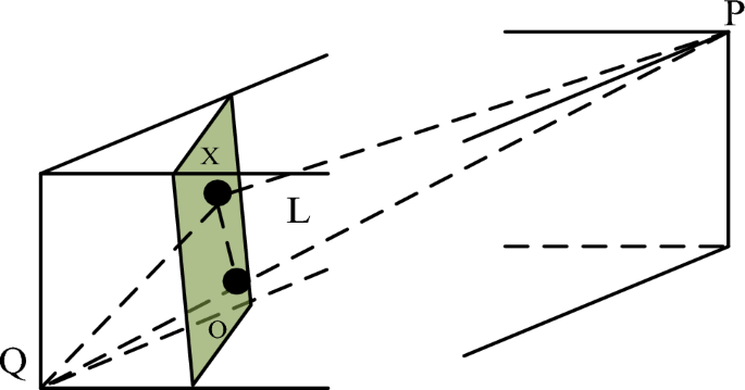
Vertical distance from any level X to the perfect resolution level.
As illustrated in Fig. 4, the idea of vertical distance refers back to the straight-line distance from any level X to the perfect resolution level P or Q. Taking the vertical distance from level X to the perfect resolution level Q for example, we derive the components. Since the road XO is perpendicular to the road PQ, we receive Eq. (15):
$$left{ {start{array}{*{20}c} {left( {QX} proper)^{2} – left( {QO} proper)^{2} = left( {XP} proper)^{2} – left( {OP} proper)^{2} } {QO + OP = PQ} finish{array} } proper.$$
(15)
The distance between level O and level Q is the vertical distance from X to the perfect resolution level Q, expressed as:
$$QO = frac{{left( {QX} proper)^{2} + left( {PQ} proper)^{2} – left( {XP} proper)^{2} }}{2PQ}$$
(16)
Similarly, the space from level O to level P is the vertical distance from X to the perfect resolution level P, expressed as:
$$OP = frac{{left( {XP} proper)^{2} + left( {PQ} proper)^{2} – left( {XQ} proper)^{2} }}{2PQ}$$
(17)
In this paper, the orthogonal projection technique is used to rank the schemes, and the fundamental steps are as follows.
Step 1: The normalized matrix of the profit attributes and the normalized matrix of the associated fee attributes are constructed as follows:
$$overline{u}_{ij}^{okay} = frac{{mu_{ij}^{okay} }}{{sumlimits_{{textual content{i = 1}}}^{m} {upsilon_{ij}^{okay} } }},overline{upsilon }^{okay}_{ij} = frac{{upsilon_{ij}^{okay} }}{{sumlimits_{{textual content{i = 1}}}^{m} {mu_{ij}^{okay} } }},i in 1,2,…,m;j in I_{1} ,{textual content{profit attribute}}$$
(18)
$$overline{u}_{ij}^{okay} = frac{{{1 mathord{left/ {vphantom {1 {upsilon_{ij}^{okay} }}} proper. kern-0pt} {upsilon_{ij}^{okay} }}}}{{{1 mathord{left/ {vphantom {1 {sumlimits_{{textual content{i = 1}}}^{m} {mu_{ij}^{okay} } }}} proper. kern-0pt} {sumlimits_{{textual content{i = 1}}}^{m} {mu_{ij}^{okay} } }}}},overline{upsilon }_{ij}^{okay} = frac{{{1 mathord{left/ {vphantom {1 {mu_{ij}^{okay} }}} proper. kern-0pt} {mu_{ij}^{okay} }}}}{{{1 mathord{left/ {vphantom {1 {sumlimits_{{textual content{i = 1}}}^{m} {upsilon_{ij}^{okay} } }}} proper. kern-0pt} {sumlimits_{{textual content{i = 1}}}^{m} {upsilon_{ij}^{okay} } }}}},i in 1,2,…,m;j in I_{2} ,{textual content{value attribute}}$$
(19)
Step 2: Determine the attribute weight (omega_{j} (t_{okay} )) of various time durations utilizing Model (M-1), Model (M-2), and Eq. (9). Then, the weighted intuitionistic fuzzy matrix, (hat{A}(t_{okay} ) = (hat{A}_{ij}^{okay} )_{m occasions n} = (omega_{j}^{okay} hat{A}_{ij}^{okay} )_{m occasions n}), is obtained. Model (M-4) is used to resolve the time collection weight vector, (eta_{{t_{okay} }} = (eta (t_{1} ),eta (t_{2} ),…,eta (t_{p} ))^{T}), and the dynamic intuitionistic fuzzy weighted geometry (DIFWG) operator in Definition 6 is used to combination the weighted intuitionistic fuzzy resolution matrix of every time interval, and the dynamic intuitionistic fuzzy complete resolution matrix (hat{A}(t_{okay} ) = (hat{A}_{ij}^{okay} )_{m occasions n}) is obtained, the place,
$$start{gathered} R = (r_{ij}^{{}} )_{m occasions n} = (sigma_{ij}^{{}} ,tau_{ij}^{{}} )_{m occasions n} = left[ {begin{array}{*{20}c} {(sigma_{11}^{{}} ,tau_{11}^{{}} )} & {(sigma_{12}^{{}} ,tau_{12}^{{}} )} & {…} & {(sigma_{1n}^{{}} ,tau_{1n}^{{}} )} {(sigma_{21}^{{}} ,tau_{21}^{{}} )} & {(sigma_{22}^{{}} ,tau_{22}^{{}} )} & ldots & {(sigma_{2n}^{{}} ,tau_{2n}^{{}} )} vdots & vdots & ddots & vdots {(sigma_{m1}^{{}} ,tau_{m1}^{{}} )} & {(sigma_{m2}^{{}} ,tau_{m2}^{{}} )} & ldots & {(sigma_{mn}^{{}} ,tau_{mn}^{{}} )} end{array} } right] finish{gathered}$$
Step 3: The constructive and adverse excellent options of the dynamic intuitionistic fuzzy artificial resolution matrix (R = (r_{ij} )_{m occasions n}) is set as follows:
$$r_{j}^{ + } = (sigma_{j}^{ + } ,tau_{j}^{ + } ){ = }(mathop {max}limits_{1 le i le m} sigma_{ij} ,mathop {min}limits_{1 le i le m} tau_{ij} ),(j = 1,2,…,n)$$
(20)
$$r_{j}^{ – } = (sigma_{j}^{ – } ,tau_{j}^{ – } ){ = }(mathop {min}limits_{1 le i le m} sigma_{ij} ,mathop {max}limits_{1 le i le m} tau_{ij} ),(j = 1,2,…,n)$$
(21)
Step 4: Definition 7 is utilized to calculate the space between each intuitionistic fuzzy quantity (r_{ij}) and its corresponding constructive and adverse excellent options (Eq. 22 and Eq. 23, respectively) and the space between the constructive excellent resolution and the adverse excellent resolution (Eq. 24):
$$d(r_{{^{i} }} ,r^{ + } ) = sqrt {frac{1}{2}sumlimits_{j = 1}^{n} {left[ {(sigma_{{_{j} }}^{ + } – sigma_{ij} )^{2} + (tau_{{_{j} }}^{ + } – tau_{ij} )^{2} + (pi_{{_{j} }}^{ + } – pi_{ij} )^{2} } right]} }$$
(22)
$$d(r_{{^{i} }} ,r^{ – } ) = sqrt {frac{1}{2}sumlimits_{j = 1}^{n} {left[ {(sigma_{{_{j} }}^{ – } – sigma_{ij} )^{2} + (tau_{{_{j} }}^{ – } – tau_{ij} )^{2} + (pi_{{_{j} }}^{ – } – pi_{ij} )^{2} } right]} }$$
(23)
$$d(r^{ + } ,r^{ – } ) = sqrt {frac{1}{2}sumlimits_{j = 1}^{n} {left[ {(sigma_{{_{j} }}^{ – } – sigma_{{_{j} }}^{ + } )^{2} + (tau_{{_{j} }}^{ – } – tau_{{_{j} }}^{ + } )^{2} + (pi_{{_{j} }}^{ – } – pi_{{_{j} }}^{ + } )^{2} } right]} }$$
(24)
Step 5: The vertical distance between every scheme and the adverse excellent resolution is calculated through the use of Eq. (25).
$$V_{i}^{ – } = frac{{d^{2} (r^{ + } ,r^{ – } ) + d^{2} (r_{i} ,r^{ – } ) – d^{2} (r_{i} ,r^{ + } )}}{{second(r^{ + } ,r^{ – } )}}$$
(25)
The schemes may be ranked based on the vertical distance. The bigger the vertical distance (V_{i}^{ – }), the farther the scheme (S_{i}) is from the adverse excellent resolution and the higher the scheme is (S_{i}).
Proposed strategy based mostly on subject principle
Concept and definition of subject mannequin
In physics, the sector principle displays an invisible interplay and affect impact in a holistic and steady method67. In the innovation progress of an DAST innovation alliance, the relationships between the alliance and its companions even have a sure holistic attribute, and the connection between the 2 events has a continuity attribute. Therefore, this paper adopts the sector principle to research the selection technique of cooperative innovation companions for an DAST innovation alliance.
The subject supply (denoted as (O)) constitutes a DAST innovation alliance, characterised by its capability to leverage progressive belongings all through the collaborative growth course of. As established by67, the alliance’s collaborative innovation efficiency straight correlates with its progressive asset base, quantified by way of two key metrics: useful resource deployment effectivity and reserve portions. The stock of innovation assets is outlined as (M{ = }(m_{1} {,}m_{2} {,} ldots {,}m_{n} )), the place (n) represents the spatial dimension of innovation assets. Any innovation useful resource ought to fulfill the situation: (0 le m_{i} le 1). When (m_{i} { = }1), it signifies that this innovation useful resource meets the necessity of cooperative innovation, and when (m_{i} { = 0}), it signifies that this innovation useful resource doesn’t meet the wants of cooperative innovation. The utilization price of innovation assets is outlined as (P{ = }(p_{1} {,}p_{2} {,} ldots {,}p_{n} )), and (0 le p_{i} le 1), the place (p_{i}) represents the utilization of the useful resource inventory (m_{i}). The provide of innovation assets will change dynamically in numerous time durations because of the inside elements of DAST innovation and the exterior surroundings.
Therefore, when incorporating temporal issues into the evaluation framework (with the research interval outlined as (T{ = }(t_{1} {,}t_{2} {,} ldots {,}t_{n} ))), the collaborative innovation functionality stage of the DAST innovation alliance, denoted as (Q_{T}), may be mathematically represented by way of the next formulation:
$$Q_{T} = M occasions P_{T} = sumlimits_{i = 1}^{n} {m_{i} p_{i} }$$
(26)
During the cooperative innovation means of an DAST innovation alliance, there’s useful resource complementarity between the candidate companions and the innovation alliance. Setting the useful resource stock of the candidate partner as (H{ = }(h_{1} {,}h_{2} {,} ldots {,}h_{n} )), the demand for the assets as (overline{M}), and the house saturation diploma as (tilde{M}{ = (}overbrace {{{1,1,}…{,1}}}^{n})), the cooperative innovation functionality high quality of the candidate partner, (q_{T}), may be expressed as:
$$q_{T} { = (}(tilde{M} oplus overline{M}) cap H) occasions P_{T} = sumlimits_{i = 1}^{n} {[(1 oplus m_{i} )} wedge h_{i} ]p_{i}$$
(27)
The depth of the collaborative innovation functionality subject describes the magnitude of affect exerted by subject sources on the DAST innovation alliance inside particular areas of this subject. Field energy reveals an inverse relationship with distance from the supply, the place higher proximity corresponds to stronger subject results. The directional vector of this collaborative innovation functionality subject, denoted as (E_{T}), originates at potential companions and terminates on the subject supply. (E_{T}) is set by way of the components offered under:
$$E_{T} { = }frac{{K_{T} Q_{T} }}{{R_{T}^{2} }}$$
(28)
the place (K_{T}) is the cooperative innovation functionality impact produced by the DAST innovation alliance and another partner at totally different time factors, and (R_{T}) is the radius of the cooperative innovation functionality at totally different time factors. In the present collaborative innovation surroundings, with the recruiting of a candidate partner, the rise of the alliance’s innovation high quality introduced by an innovation useful resource, may be expressed as (I_{T}), and (K_{T}) may be calculated utilizing the next equation:
$$K_{T} { = }frac{{I_{T} }}{{(Q_{T} + q_{T} )}}$$
(29)
The gravitational power related to collaborative innovation capability signifies the extent of attraction or acknowledgment that a area supply holds towards the progressive capabilities of potential companions. This gravitational impact, denoted by (F_{T}), is mathematically represented as:
$$F_{T} { = }E_{T} occasions q_{T} = frac{{I_{T} Q_{T} q_{T} }}{{(Q_{T} + q_{T} )R_{T}^{2} }}$$
(30)
The collaborative innovation capability radius ((R)) serves as a dynamic variable that holistically evaluates potential companions’ {qualifications} and competencies67. This radius parameter is derived from assessing the candidate’s innovation potential by way of a dynamic intuitionistic fuzzy decision-making framework incorporating temporal dimensions and orthogonal projection evaluation. The computational mannequin integrates multidimensional analysis standards that quantify each static attributes and evolving capabilities inside collaborative innovation techniques.
Assuming the competence and capability of the first supply is (C_{f}), whereas the substitute collaborator’s proficiency and potential are (C), the collaborative innovation radius may be mathematically expressed as follows:
$$R_{T} { = 1 + }C_{f} – C,C in [0,1]$$
(31)
The high quality and potential of (R_{1}) location within the subject is outlined as (C_{1}), (C_{f} in [C_{1} ,1]), and the standard and potential of an DAST innovation alliance is 1 ((C_{f} { = }1)). Then, the radius of the cooperative innovation potential is (R_{T} { = 2} – C). To facilitate the next dialogue and evaluation, the sector of cooperative innovation functionality on this research is split into 4 totally different sections proven in Fig. 5: ((0,R_{1} ]) is the robust cooperative innovation functionality zone, ((R_{1} ,R_{2} ]) is the medium cooperative innovation functionality zone, ((R_{2} ,R_{3} ]) is the weak cooperative innovation functionality zone, and ((R_{3} ,infty ]) is the non-cooperative innovation functionality zone. From this Fig. 5, digital coil represents the radiation vary of subject energy with totally different cooperative innovation potential, and (delta_{1} ,delta_{2} ,delta_{3} , cdots ,delta_{8}) characterize the choice companions in numerous circles.
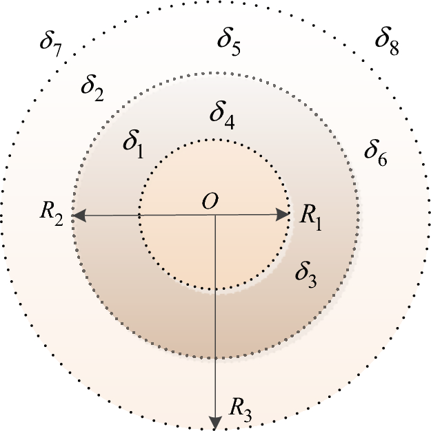
Field mannequin of the cooperative innovation functionality.
The willingness resistance is the chance and danger value of a candidate partner to affix an DAST innovation alliance. Setting (Z_{1}) as the chance value and (Z_{2}) as the chance value, the willingness resistance of a candidate partner may be expressed as:
$$F_{TW} { = }Z_{1} + Z_{2}$$
(32)
The vital situation for a candidate partner to enter or exit the innovation alliance is as follows: the radius of cooperative innovation potential, (R_{T}), is equal or smaller than the radius threshold (varphi_{T}), ((R_{T} le varphi_{T})) and gravity of the cooperative innovation potential, (F_{T}) is equal or higher than the gravity threshold (xi_{T}), and equal or higher than the resistance (F_{TW}), ((F_{T} ge xi_{T}) and (F_{T} ge F_{TW})).
Dynamic attribute evaluation for the partner selection of DAST innovation alliances
During the formation and evolution of DAST innovation alliances, enhancing collaborative innovation efficacy necessitates periodic partner renewal and structural adaptation. To optimize alliance efficiency, member composition requires dynamic refinement by phasing out underperforming collaborators whereas actively recruiting certified entities that align with alliance requirements. The partner selection mechanism inside DAST alliances demonstrates evolving parameters, the place innovation capability metrics and area experience benchmarks bear steady recalibration based mostly on shifting operational necessities. This necessitates establishing versatile analysis frameworks that account for technological developments and market fluctuations, making certain sustained alignment between partner capabilities and alliance aims.
Defining (N_{t}) because the partner who withdraws from an DAST innovation alliance on the (t)th time interval, the standard of the cooperative innovation functionality may be expressed as:
$$Q_{t + 1} { = }Q_{t} + q_{t} – N_{t}$$
(33)
The dynamic change within the subject energy of the innovation functionality of the DAST innovation alliance within the (t{ + }1)th time interval may be outlined as:
$$E_{t + 1} = frac{{[K_{t + 1} {(}Q_{t} + q_{t} – N_{t} )]}}{{R_{t + 1}^{2} }}$$
(34)
Hence, the sections of the cooperative innovation functionality subject can be adjusted accordingly, as proven in Fig. 6.

Dynamic adjustments of the sections of the cooperative innovation functionality.
The companions positioned within the inside sections of the cooperative innovation functionality subject have robust cooperative innovation functionality fields and can totally combine and use the assets of the DAST innovation alliance to advertise additional enchancment of their cooperative innovation capabilities. With vital enchancment within the stage of companions’ innovation performances, their willingness resistance might change in a number of folds. The willingness resistance may be expressed as (F_{(t + 1)W} { = }chi M_{t + 1})68. A candidate partner positioned near the outer part of the cooperative innovation functionality subject is influenced by each the cooperative innovation functionality gravity, (F_{T}), and the willingness resistance, (F_{TW}), as proven in Fig. 7.

Internal and exterior forces of an DAST innovation alliance based mostly on the cooperative innovation subject.
Dynamic selection process of DAST innovation alliances
The cooperative innovation subject mannequin is carried with the next steps:
Step 1: The cooperative innovation potential of every partner is obtained by the built-in fuzzy orthogonal projection strategy technique based mostly on resolution guidelines.
Step 2: Based on the analysis of the standard and capabilities of the DAST innovation alliance and its candidate companions, the sector energy, attraction, radius, and resistance based mostly on innovation potential are calculated by Eqs. (28–34).
Step 3: The radius threshold worth and attraction threshold worth are calculated based mostly on knowledgeable session.
Step 4: Based on the set off level, a number of potential companions are eradicated. The remaining candidates are subsequently ranked based on their resultant power values, from which a number of companions are chosen to affix the DAST innovation alliance.
Figure 8 presents processes used for DAST innovation alliance partner selection. In the built-in time-weighted fuzzy orthogonal projection technique, main steps embrace: (a) the partner selection index framework of the DAST innovation alliance is structured based mostly on subject principle; (b) cooperation aspiration of other companions is obtained utilizing fuzzy set principle with innovation qualities (useful resource complementary stage and knowledge-sharing stage) and innovation talents(cultural similarity, risk-sharing potential and cooperation compatibility potential); (c) standards weight vectors are decided by combining grey correlation evaluation with the utmost deviation strategy and entropy measure technique; (d) time weight vectors are additionally calculated by entropy measure technique with a multi-objective optimization mannequin; (e) innovation analysis scores of alternate options are obtained utilizing orthogonal projection technique. In the cooperation innovation subject mannequin for partner selection based mostly on subject principle, main steps embrace: (a) complementary assets set for DAST innovation are structured by specialists technique; (b) the cooperation innovation potential of alternate options and complementary assets set is remodeled into the radius of innovation subject and the cooperation innovation qualities of alternate options, respectively; (c) subject energy of the cooperation innovation subject is calculated through the use of proposed subject technique; (d) gravitational power and willingness resistance of alternate options in cooperation innovation subject, respectively; (e) resultant power of alternate options and alternate options rating is obtained, and (f) a number of innovation companions are really helpful to the DAST alliance managers.
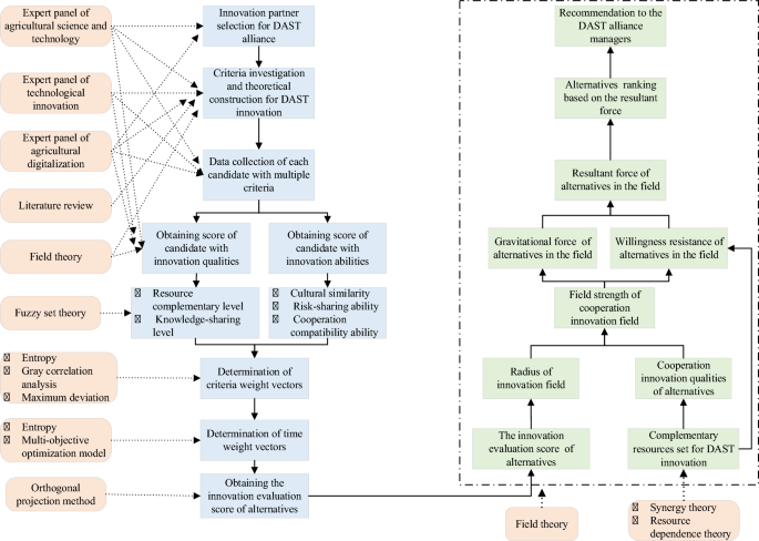
Dynamic selection process of DAST innovation alliance.